Download Package of Charles University Implementation of High Cycle Accumulation Model

Download Package of Charles University implementation of high cycle accumulation model

Authors: T. Kadlíček (2022) with contributions of M. Ochmański, D. Mašín and J. Duque

Related publications:

Kadlíček, T., Ochmański, M., Mašín, D. and Duque, J. (2022) Report on Charles University implementation of high cycle accumulation model

1 file(s) 2.34 MB

Please login to download

Niemunis, A., Wichtmann, T., Triantafyllidis, Th. (2005): A high-cycle accumulation model for sand, Computers and Geotechnics, Vol. 32, Nr. 4, S. 245-263

1 file(s) 0.25 KB

Please login to download

Associated software and constitutive models:

+

Abaqus

SoilModels Admin|13.1.201815.9.2021|Simulation Software|1 |

Views 19,329

The Abaqus Unified FEA product suite offers powerful and complete solutions for both routine and sophisticated engineering problems covering a vast spectrum of industrial applications.

26 likes Read more

+

Tochnog Professional – Free FEM Code

Dennis Roddeman|12.1.201815.9.2021|Simulation Software|0 |

Views 3,366

Tochnog Professional is a free Finite Element program offering a wide variety of geotechnical and mechanical options; modern material laws including the most recent rate independent and viscous hypoplasticity models.

4 likes Read more

+

A High-Cycle Accumulation Model for Sand (Niemunis et al., 2005)

SoilModels Admin|6.9.20226.9.2022|Constitutive Models|0 |

Views 887

A high-cycle explicit model for the accumulation of strain in sand due to small cyclic loading. The dependence of the accumulation rate on stress, void ratio, cyclic history and the type of loading is considered. In particular, the ovality and the polarization of the strain path during a cycle are taken into account.

4 likes Read more

Readme:

This ReadMe file explains structure of the High Cyclic Accumulation model (HCA) implementation introduced by Wichtmann and Niemunis.
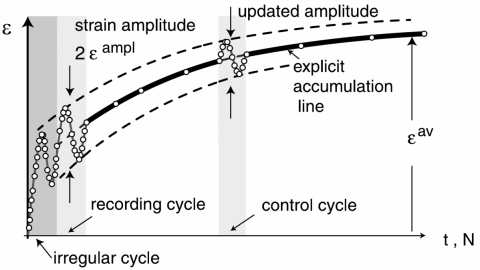
The implementation is structured as required by Abaqus' User MATerial (UMAT). The implementation distinguishes between implicit and an explicit part of a cyclic loading.
The implicit part performs a strain loop in its full length and subsequently calculate properties necessary for the explicit simulation with the HCA model.
The implementation currently contains these constitutive models:
- Wolffersdoff's hypoplatic sand model (1996)
- The high cyclic accumulation model for sand according to the Wichtmann habilitation (2016)
- The high cyclic accumulation model for clay according to the Wichtmann habilitation (2016)
- Masin's hypoplastic clay model. It is an external model and it is not influenced by settings in "umatConstants.f90"
The implementation contains these files:
- umat.f90
- umat_hyposand.f90
- umat_HCA.f90
- operations.f90
- hypoplasticity.f90
- highCyclicAccumulation.f90
- RungeKutta.f90
- umatConstants.f90
- umat_hcea.for - independent

umat.f90
- calls the implicit (umat_hyposand.f90) or explicit (umat_HCA.f90) part of the simulation in an accordance with setting defined in the "umatConstants.f90".
- storing the strain loop points and calculation of the fourth order strain amplitude tensor "Aeps" and polarization "PI" is executed at the "kstep" designated in
"umatConstants.f90". The strain loop points are stored in the state variable vector "statev". The vector thus should be large enough to accommodate reasonable number
of increments performed during the simulation. If the number of stored strain loop points exceeds length of the vector statev, the strain loop point with the shortest
distance is deleted to accommodate new strain loop point.
- the polarization PI of the HCA model is commented, i.e., omitted from the simulation. It can be switched on, however, enough space should be allocated
in the "statev" vector to store "polarization PI". As stated in the Wichtmann habil, polarization can be omitted from the most of engineering problems.

umat_hyposand.f90 & umat_HCA.f90
- the file transfers vector notation of stress and strain to tensor notation and call RKF integration. Later exports tangent stiffness matrix of the increment "ddsdde".
- both files can be used independently of the file umat.f90 if properly modified

operations.f90
- the file contains numerous functions performing or supporting algebraical or tensorial operations.

hypoplasticity.f90
- the file contains functions evaluating scalar and tensorial variables of the hypoplastic sand model. The function called "incrementHS" orders these function in the specific
order to calculate one parameter of the RKF integration.
- implementation of other hypoplastic models should be done here.

highCyclicAccumulation.f90
- the file contains functions evaluating scalar and tensorial variables of the HCA models. The function called "incrementHCA" orders these function in the specific
order to calculate one parameter of the RKF integration.

RungeKutta.f90
- this file performs integration of the differential equation for all directly implemented models. Decision of the integration are made base on the key names:
- HSI - hypoplastic sand mode with intergranular strain (Wolffersdoff's model)
- HCA - High Cyclic Accumulation model for sand/clay
- further implementations should follow this example

umatConstants.f90
- this file contains "parameters" for various parts of the calculation.

- general settings are defined first:
* modelType (sand/clay) - this sets whether the "sand" or "clay" model is considered during a simulation.
* calcJacobian (YES/NO) - this setting provides an option to directly calculate jacobian "ddsdde". If the option "NO" is selected,
ddsdde is calculated based on the 4th order elastic stiffness tensor L. Direct calculation often provides lower error estimation,
however, ddsdde based on L gives more stable iteration process. Tochnog requires full ddsdde matrix even for 2D simulation.
Therefore, it might be more advantageous to fill dstran vector with homogeneous dstrain increment, e.g. dstran = 1e-5, in the case
of the direct calculation.
* notation (VOIGT/UMAT/TOCHNOG) - "UMAT" notation should be used in the most cases. "TOCHNOG" notation is redundant even for the simulation in TOCHNOG.
Option "VOIGT" can be used in some cases.
* nHypoParam (14/21) - the hypoplastic clay and sand model requires different number of parameters. This has to be set correctly for a successful calculation
* initIncrement(0/1) - some software starts counting of the first increment "kinc" from "0" and some from "1". This has to be remembered during HCA simulation.
- the "Incremental driver" developed by A. Niemunis which was used for a verification of the implementation starts counting from "1"(Might have been modified).

- the parameters driving integration of the RKF method are defined separately for the hypoplastic model sand and HCA model as they require a different level of a precision.:
* maxAllowedStep_Hypo/maxAllowedStep_HCA - defines maximal allowed step size h for the hypoplastic/HCA model in RKF
* minAllowedStep - defines minimal allowed step size h
* RKF_TolY_Hypo,/RKF_TolY_HCA - RKF tolerance for the hypoplastic/HCA model

- minimal stress setting is provided as in some cases empty ddsdde can be provided upon stresses oscillation around mean stress "p = 0 kPA".
Therefore minimal stress setting is provided:
* minAllowedStress - Minimal stress at which RKF is interrupted. It also defines minimal stress (compression) considered for I1 in calculations. This improves stability of a calculation.
* resetLowStressLevel (YES/NO) - If set to YES, diagonal stress elements are set to "minAllowedStress" when I1 > minAllowedStress (copression)

- the intergranular strain requires further characteristics
* numSmallStrainSteps - defines number of steps defined for the whole small strain magnitude R. This significantly decrease the step size h of the integration.
The decrease is omitted if the small strains and strain loading directions are aligned.
* smallStrainDirTol - Angle at which the small strains and strain loading directions are considered as aligned.
- In (Niemunis, 1997), progressive increase of the step size is proposed with alignment of the small strains.
* dStrainMin_Hypo - maximal strain increment magnitude for the HSI model ||dstrain|| < dStrainMin_Hypo

- the position of the state variables in the vector "statev" is defines as a type "StateVariablePossiotion". Similarly the position of the models parameters
in the vector "props" is defined as the type "MaterialPossiotion". Position of the state variables and parameters in the related vectors "MUST NOT" be defined elsewhere
in the code.

- the "ksteps" designated for the calculation of the tensorial strain amplitude "Aeps" and the "polarization PI" are defined in the vectors:
* implicitLoop2recAeps
* implicitLoop2recPI

- the strain loop is recorded during the whole step and "Aeps" or "PI" are evaluated continuously during the designated "kstep". This leads to a decrease in a calcualtion speed
during these steps.

- the position of the implicit/explicit loading are defined by "loadingConditions". This array defines number and order of the implicit and explicit cyclic loadings.
The first row in the array defines type of loading with a key number "1" (implicit) or "2" (explicit). The second row defines a number of implicit cycles by an integer number.
The explicit loading is ALWAYS defined by number "1" as the number of explicit cycles is defined by time (dtime).

- examples of loading setting for numerical calculations:
Example 1 - FEM analysis, cyclic loading in one direction (polarization is nor required)
- step 1 - monotonic loading - construction phase
- step 2 - monotonic loading - construction phase
- step 3 - implicit loop - first irregular cycle
- step 4 - implicit loop - the regular cycle for calculation of the cyclic characteristics
- step 5 - cyclic loading - explicit loading

-settings
integer, dimension(1), parameter :: implicitLoop2recAeps = (/4/)
integer, dimension(1), parameter :: implicitLoop2recPI = (/50/)
integer,dimension(2,2), parameter :: loadingConditions = reshape( (/1, 2, &
4, 1/),(/2,2/))

Example 2 - FEM analysis, preloading in the first direction, subsequent cyclic loading in the second direction
- step 1 - monotonic loading - construction phase
- step 2 - monotonic loading - construction phase
- step 3 - implicit loop - first irregular cycle in the first direction
- step 4 - implicit loop - the regular cycle for calculation of the polarization PI in the first direction
- step 5 - implicit loop - first irregular cycle in the seconds direction
- step 6 - implicit loop - the regular cycle for calculation of the tensorial strain amplitude
- step 7 - cyclic loading - explicit loading

-settings
integer, dimension(1), parameter :: implicitLoop2recAeps = (/6/)
integer, dimension(1), parameter :: implicitLoop2recPI = (/4/)
integer,dimension(2,2), parameter :: loadingConditions = reshape( (/1, 2, &
6, 1/),(/2,2/))

Example 3 - FEM analysis, preloading in the first direction, cyclic loading in the second direction, control cycle, cyclic loading, control cycle, cyclic loading,
- step 1 - monotonic loading - construction phase
- step 2 - monotonic loading - construction phase
- step 3 - implicit loop - first irregular cycle in the first direction
- step 4 - implicit loop - the regular cycle for calculation of the polarization PI
- step 5 - implicit loop - first irregular cycle in the seconds direction
- step 6 - implicit loop - the regular cycle for calculation of the tensorial strain amplitude
- step 7 - cyclic loading - explicit loading
- step 8 - implicit loop - first irregular cycle for the control cycle
- step 9 - implicit loop - the regular cycle for calculation of the tensorial strain amplitude
- step 10- cyclic loading - explicit loading
- step 11- implicit loop - first irregular cycle for the control cycle
- step 12- implicit loop - the regular cycle for calculation of the tensorial strain amplitude
- step 13- cyclic loading - explicit loading

-settings
integer, dimension(3), parameter :: implicitLoop2recAeps = (/6,9,12/)
integer, dimension(1), parameter :: implicitLoop2recPI = (/4/)
integer,dimension(6,2), parameter :: loadingConditions = reshape( (/1, 2, 1, 2, 1, 2, &
6, 1, 2, 1, 2, 1 /),(/6,2/))
The number of explicit cycles has to be defined by the variable "Time" for each step with explicit loading!

Example 4 - Single element analysis with hypoplastic sand model
- step 1 - monotonic loading
- step 2 - cyclic loading

-settings
integer, dimension(3), parameter :: implicitLoop2recAeps = (/6,9,12/) - do not have to be changed as Aeps is calculated in 6th, 9th and 12th step
integer, dimension(1), parameter :: implicitLoop2recPI = (/4/) - dont have to be changed as PI is calculated in 4th step
integer,dimension(1,2), parameter :: loadingConditions = reshape( (/1, &
2 /),(/1,2/))